You might experience a situation where a supplier sends you an updated list of products with changes to existing and new products.
Unfortunately, it, oftentimes, isn't explicitly stated which products are new and which already exist, and our import function cannot import both categories at once.
Therefore, we have created this comprehensive guide to help you out when you receive a new supplier list.
Prepare Your Files
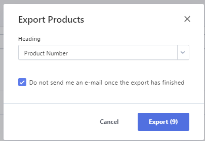
Start by ensuring that you have the necessary data ready to begin with. In addition to the file you've received from the supplier, you also have to download a product list from Rackbeat.
Here, I have only selected the "product numbers" as a column since it's the only relevant information for me in this case.
Merging Files
Once both files are ready, you need to merge them without losing crucial parts of the product numbers. This goes for all product numbers that start with "0" as they are automatically removed when you export a file to Excel.
We can't have that!
So, to avoid this, go to the file you received from the supplier and find "Data" at the top.
Now, click on "From Text/CSV"
Next, select the file. Once this is done, you'll see a window that looks something like this:
If you have a product number that begins with 0, you'll realize that some of the product numbers no longer contain the desired "0", as shown in the image above.
To correct this, find the option that says "Data Type Detection" and change it to "Based on the entire dataset." See below:
Once selected, you should be able to see that the product numbers now contain a 0 in your overview:
Note that the item numbers starting with "0" are suddenly visible! Now you can click on "Transform Data."
A new window will open, and here you can make corrections to the column. If it looks correct, click on "Close & Load."
This creates a new tab in your Excel sheet with the item numbers from Rackbeat retaining the "0." So far, so good!
In this case, I've named the tab "Rackbeat product list" and added another column called "Exist in Rackbeat" where each line has the text "Exist in RB." This text is important because it will appear in the column that will tell us whether the item exists or not.
Data Comparison
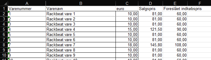
Now that we have all the data in one file, we need to compare the data to separate what's new and what already exists. So, let's switch to the main tab, the one with the products you received from your supplier.
Our supplier list looks like this:
In column "G," I've created a title called "Already Exists" (Note that it won't necessarily appear in your column G).
Here, we need to use the XLOOKUP function that Excel provides, as we will use it to compare our two datasets.
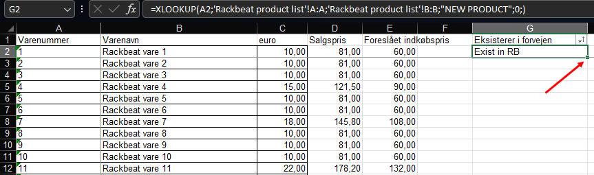
The formula I've created looks like this:
=XLOOKUP(A2,'Rackbeat product list'!A:A,'Rackbeat product list'!B:B,"NEW PRODUCT",0)
It may look a bit confusing when you first take a look at it, so let's walk through each step of the function:
The formula itself is called =XLOOKUP(Lookup_value; Lookup_array; Return_array; [If_not_found]; [Match_mode]; [Search_mode]) and it allows you to search for a value and return another value related to the searched value.
Let's break it down into individual functions:
- Lookup_value = What value are we looking for? In this example, we are searching for the value in A2, which is "1".
- Lookup_array = Where should we look for the above value? In this example, we're searching the entire column with item numbers from Rackbeat, so you need to go to the tab we created and select the whole column. In the example of the formula I provided above, you can see that I've chosen "'Rackbeat product list'!A:A;".
- Return_array = If it finds the value it's looking for, which column should it return the data from? This is where we need to use the column we created earlier, called "Exist in Rackbeat," because that's the data we want to display if it finds the right value. So here, I've selected "'Rackbeat product list'!B:B;".
- [If_not_found] = We need to specify what we want it to show if it doesn't find the value. I've decided that it should write "NEW PRODUCT" because it means that the item doesn't already exist in Rackbeat. I've done that by typing "NEW PRODUCT," and do remember to use quotation marks when entering the text.
- [Match_mode] = Here, we have to specify how precise we want it to be. I've chosen "0" for EXACT MATCH.
- [Search_mode] = Here, we can specify how it should search. I've skipped this part and just closed with the final parenthesis.
So, it should look like this for you. To expand it to the entire column, you can double-click on the small square in the lower right corner when you have selected the cell. (See the red arrow)
Afterwards, it should look like this:
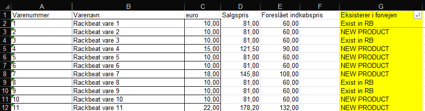
(I've highlighted it in yellow to emphasize the column).
Then, I filtered the column by selecting the title "Already Exists" and clicking on "Sort & Filter."
Once that's done, I clicked on the new box next to the title:
Finally, you can choose what you want to see and transfer that data to the sheets you need to work with. 🌞
Thus, we reached the conclusion to our supplier import guide 🙌